EBL Models¶

The EBL module come from the ebltable git repository (see https://github.com/me-manu/ebltable)

Supported Models¶

Currently there is 5 models supported :

Franceschini, A., Rodighiero, G., & Vaccari, M.2008, A&A, 487, 837 . http://adsabs.harvard.edu/abs/2008A%26A…487..837F

Finke, Razzaque, & Dermer, 2010, ApJ, 712, 238 . http://adsabs.harvard.edu/abs/2009arXiv0905.1115F

Dominguez, A., Primack, J.R., Rosario, D. J., et al. 2011, MNRAS, 410, 2556 . http://adsabs.harvard.edu/abs/2011MNRAS.410.2556D

Inoue, Y., Inoue, S., Kobayashi, M. A. R., et al. 2013, ApJ, 768, 197 http://adsabs.harvard.edu/abs/2013ApJ…768..197I

Kneiske, T. M., & Dole, H. 2010, A&A, 515, A19 http://adsabs.harvard.edu/cgi-bin/bib_query?arXiv:1001.2132

Each model is read using

from ebltable.tau_from_model import OptDepth as OD
tau = OD(model = 'inoue')
# Source redshift
z   = 0.2
# array with energies in TeV
ETeV = np.logspace(-1,1,50)

# calculating the optical depth for a redshift z and TeV energies
# this returns a two dimensional array with dimensions
# of the redshift array times dimensions of the energy array.
# Since z is a scalar here, it will return a 1 x 50 dim array.
t = tau.opt_depth_array(z,ETeV)

Flux correction¶

For correction of the flux, you can then compute

import numpy
correction = numpy.exp(-1. * t[0])

Example¶

The example script can help to understand and will produce this plot

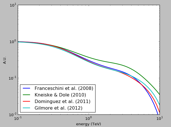
Exemple of flux in A.U. corrected with the supported models. This plot has been generated by the script ExempleEBL.py